Creating
shaded-relief, hypsometrically tinted, 250K topos for CASARA navigators
by Morgan Hite (mjh@hesperus-wild.org)
last updated 29-Nov-2010
Download maps
I'll give the most current process for making the maps first. At the bottom,
I'll give obsolete methods.
In this process I create a shaded relief version of an NTS 250K topo sheet (Canada),
with elevation shading similar to a VNC chart.
Examples pictured below are from sheet 093L (Smithers, British Columbia).
In these instructions, I'll assume (because this is what I have) that you have
one machine with all the software installed on it, and a server where the original
data and the finished images are stored. If you have a single workstation where
all files are stored, ignore my references to "the server" because you'll save
everything locally.
Software packages used in the process are:
- Global Mapper ($ http://www.globalmapper.com/)
- MapInfo ($ www.mapinfo.com)
- Vertical Mapper -- an add-on to MapInfo ($ www.tetrad.com/)
- 3DEM v 18.7 This wonderful piece of free software is now hard to find, particularly
this version, which was not the last version of 3DEM released. You want this
specific versio,n as it permitted a larger magnification before export. You
can download it from me here (5MB).
- GeotiffExamine (originally free from mentor software; now
apparently no longer available--however, other geotiff tag reading
packages certainly must be)
- 602Photo (originally shareware from http://602software.com. It's
been discontinued, however it's still available at
http://www.archive.org--search on '602Photo'. This version only
functions for 30 days, but then you can uninstall and re-install and
get another 30 days.)
- OziExplorer ($ -- this is just for printing the final images)
I would welcome any workarounds to make the entire process use free
software, but at present I have access to licenced versions of these
packages, so using them makes sense for me.
There is a surprising number of different pieces of software in use
here. I suspect the whole thing could be done in ArcMap, but it exceeds
my knowledge of ArcMap, so I use what I know.
Contents
- Creating
shaded-relief, hypsometrically tinted, 250K topos
- Original data
- Joining the two DEM
halves
- Building hypsometric
regions
- Overlaying
hypsometric regions on the original 250K topo
- ArcMap method
- Applying shaded
relief with 3DEM
- Tweak image and
manufacture world file
- GeotiffExamine
- Tweak image
- Calibrating in
OziExplorer
- Mosaic with adjacent
maps
- Now obsolete methods
- Making hypsotint polygons
- Global Mapper Method
- Oasis/montaj method
- Overlaying lakes polygons in
MapInfo
- Saving final results as PNG
- Saving final results as Geotiff
from MapInfo
- Merging in MapMerge
- Remaining issues
- Need to calibrate
final result
- Mosaicking final
results
- Apparent topographic
reversal
- Lakes obscure some
map text
Original data
I begin with three data sets on my server for each 1:250K NTS topo
sheet: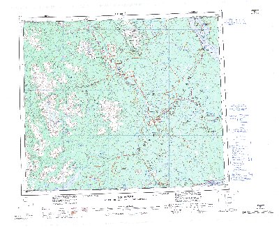
- the NTDB (National
Topographic DataBase) vector files for the
same 250K topo. These are free of charge from the appropriate
subdirectory of ftp://ftp2.cits.rncan.gc.ca/pub/bndt/250k_shp_en/
(alternatively, one can go in through www.geogratis.ca).
From this data set we will get the water bodies used below. (Note, April 2010: with the release
of CanVec data, you have a second choice. It can be downloaded
from ftp://ftp2.cits.rncan.gc.ca/pub/canvec/. However, CanVec data only comes by
the 1:50,000 mapsheet, which makes it clumsy for this use. It is almost
too detailed, and you have
to merge 16 mapsheets to get one dataset for a 1:250,000 map.)
- the DEM (digital
elevation model) for the same 250K topo, ordered
through www.geobase.ca/. The
format is CDED1. Free registration is required at this site. Each ZIP
archive (corresponding to a 250K map) consists of two files, a DEM for
the East half and a DEM for the west half.
Joining the two DEM
halves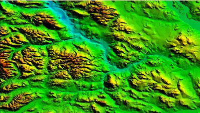
CDED dems come as two files: east half and west half. You need to unify
them into a single file so 3DEM can read them.
Read both halves of the DEM into Global Mapper and export as a single
DEM file (still on the server). Export with File>Export Raster and
Elevation Data>Export DEM...
I use Global Mapper rather than the free software package MicroDEM
because 3DEM does not always accept MicroDEM's output.
Note that within Global Mapper the projection of the DEM is Lat/Long,
and it is important not to change its projection to UTM at this point
-- 3DEM expects the DEM in Lat/long.
Building hypsometric
regions
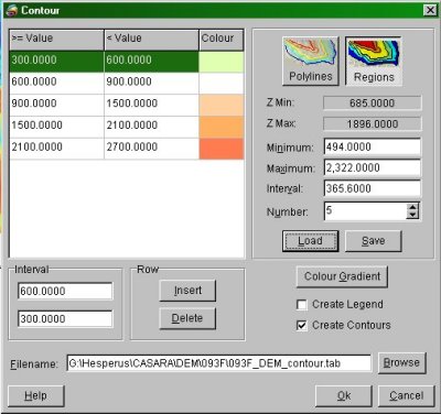
Read the unified DEM into MapInfo/Vertical Mapper (Create Grid|Import
Grid).
Create contour regions (Open Grid Manager|Contour|Regions), and write
to the server.
The contour intervals are intentionally the same as those on VNC
charts: 300, 600m, 900m, 1500m and 2100m. For coastal maps I used a
special low contour interval from 0 to 1 m which was white, to let the
sea appear as blue as possible.
As well, the colours are chosen to imitate the tints on the VNC charts.
However, in the present procedure, the colours are unimportant. You
assign colours again when you import these polygons into ArcMap.
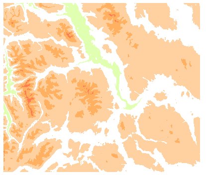
The result is a MapInfo layer of solid fill regions corresponding to
various elevation ranges ("hypsometric" tints). Note that between 600m
and 900m the regions are white, so this elevation range will overlay
as clear in the final map.
If using ArcMap to assemble layers, export to shapefile (on the server)
using the
MapInfo's "Universal Translator" (Tools>Universal Translator). It's
good to save it in the same folder as the DEM data.
It's a good idea to open the attribute table of the data in ArcMap, (or
a browser on the table in MapInfo) and make sure that the LOWER bound
for each polygon is one of the accepted values of 300, 600, etc. ArcMap
relies on these values to assign colour.
Building a lat/long grid
CASARA navigators rely on accurate longitude lines when measuring
headings. The NTS topos do not have longitude lines printed on them
(except for the east and west edges themselves) but they do have the
confusingly similar UTM lines (in blue). By printing a black grid of
lat/long lines every 15', we make the map that much more useful to the
navigator.
While ArcMap has its own tool for building a grid, it will only display
these grids in Layout View, and we need to use Map View in order to
export the image as a geotiff. The solution is to build a simple grid
of lines along the latitude and longitude lines in MapInfo, and display
it in ArcMap in the UTM projection.
With the mapper holding the DEM data open (which should still be in a
geographic or lat/longprojection) go Discover>Map grid...
Specify a grid spacing of 0.25 degrees,
and click Save As... to specify the file as <mapsheet>_grid. Save
it in the DEM data folder for this mapsheet. Click OK.
MapInfo creates a grid with labels. We're going to throw away the
labels, but the grid lines will be very useful when reprojected into
UTM by ArcMap.
Use the Universal Translator to translate the grid layer you just made
to shapefile. It will produce two shapefiles: one called
<mapsheet>_grid>polyline, which we wil use, and one called
<mapsheet>_grid>text, which we will discard.
Overlaying
hypsometric regions on the original 250K topo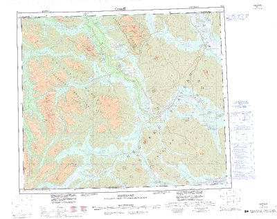
ArcMap method
Open, in this order from top to bottom, these layers from the server:
- <mapsheet>_grid_polyline (the lat/long grid) from the DEM folder for this mapsheet. (line
width 0.30, colour black).
- water_b_a.shp ("water bodies areas") from the NTDB folder for this
mapsheet (50% transparency, RGB: 151/219/242, with an
outline, 0.40, of 64/101/235; same as "Lake" in ArcMap). (Note,
April 2010: in CanVec data,
the corresponding layer is the "waterbodies" layer, coded as
"148xxxxx_2". Because CanVec data comes by the 1:50,000 mapsheet, if
you want to use CanVec data, you will have to merge the 16 mapsheets
together to get a single dataset
for the 1:250,000 mapsheet.)
- hypsometric tint polygons (see below for colours) from the DEM folder for this mapsheet, set
70%
transparent
- the CanMatrix image (contrast +20, brightness unchanged, no
transparency) from the CanMatrix
folder for this mapsheet. If it prompts you to make pyramids, say Yes.
The hypsometric tint polygons get the following colours (I have saved
this scheme in the DEM folder as hypsotints_v10.lyr
however if you load it you must always adjust the value for the
lowest elevation, whcih inevitably does not fall on one of the defined
values). Note that none has an outline. The Value Field is LOWER. 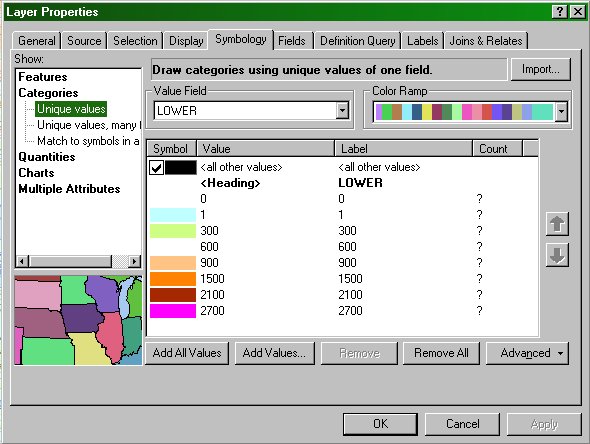
- 0 - 1 m: LOWER=0; white: RGB 255/255/255
- 1 - 300m: LOWER=1; pale blue: RGB 190/255/255
- 300-600m: LOWER=300; pale green: RGB 206/255/132
- 600-900m: LOWER=600; white: RGB 255/255/255
- 900-1500m: LOWER=900; light orange: RGB 255/195/132
- 1500-2100m: LOWER=1500; darker orange: RGB 255/130/0
- 2100-2700m: LOWER=2100; maroon: RGB 165/40/0
- 2700+m: LOWER=2700; magenta: RGB 255/0/255
Set the projection to the same as the original CanMatrix, which will be
the local UTM zone/NAD83.
Zoom to maximally fill the window (normal view). You can cut off any
collar you want, as the collar will be mostly lost when we go through
3DEM, below.
Export (File>Export Map) as TIF (Geotiff), with a dpi such that your horizontal
dimension is about 6900 pixels. I find you need quite a high dpi for this, somewhere
between 850 and 1200 depending on the size of your screen. Check Write
World File. On the Format tab, check Write Geotiff tags, choose
24-bit True Color for the Color Mode, and specify a background of white.
Save it locally. (This makes life easier
for 3DEM). This step takes a long time.
Applying shaded
relief with 3DEM
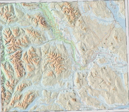 Note: the reason we run this through 3DEM is that it does something
really nice to the colours and the colour balance that I have not been
able to achieve in ArcMap alone.
Note: the reason we run this through 3DEM is that it does something
really nice to the colours and the colour balance that I have not been
able to achieve in ArcMap alone.
Read the unified DEM off the server into 3DEM
- set the projection to UTM/NAD83, which is the datum for CDED1
products
- Set the sun's azimuth to 270°, elevation 80°, shade depth
100. (Color Scale>Shaded Relief) Again, these values were arrived at
by trial-and-error. A light
source to the left works well for the eye,although as soon as one turns
the map upside down the apparent relief is reversed (see "Remaining
Issues" below)
- Turn the coordinate grid off (GeoCoordinates>Coordinate Grid
off).
- Apply the Geotiff exported from Arcmap (or Geosoft, etc.) as an
overlay (Operation>Apply/Remove Map Overlay). First you "Load" the
geotiff; then you "Accept it". 3DEM will ask for a file name to store a
helper file it creates. This step takes a
long time.
- Resize (Operation>Resize Overhead View) to the maximum zoom:
slider all the way to the right. This step takes a
long time.
- Export map image (File>Save Map Image) as Geotiff, 100%
quality. Save to the server. This file will be about 90MB. It's worth giving some thought at this
point to naming, since this will be the final file, with its
associated and similarly named TFW and MAP files. I favour <mapsheet>_SR.tif, ("SR" for
shaded relief") as in 093L_SR.tif.
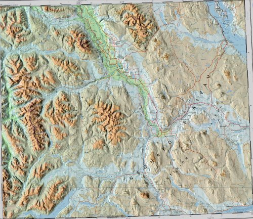
Notice that the sides of the map are not perfectly vertical.
This is because NTS maps are in UTM projections, yet paradoxically are cut along longitude lines.
Lines of longitude and UTM grid lines are only parallel in the exact
centre of each UTM zone.
So generally, and this is the case for this example map, 093L, the
lat/long grid is tilted with respect to the UTM grid.
The inconvenient result is that there are wedges of grey in the top
left and bottom right corners of the image. We'll have to crop or
mask those out later.
Create world file, tweak image
and re-write geotiff tags
GeotiffExamine
Open the geotiff with GeotiffExamine, and write the world file to the
server as well. OziExplorer will need this to automatically register
the map.
- Click Browse and find the geotiff
- Click the -> arrow button
- Click "Write World File."
Tweak image
 Open 602 Photo and read
in the geotiff.
Open 602 Photo and read
in the geotiff.
- Set brightness and contrast(Image>Brightness & Contrast, or Ctrl-K)
to
- brightness -45
- contrast +45
- Sharpen (Image> Sharpen, or Ctrl-T)
- Save. Note that when you save, 602 Photo asks this enigmatic question: "Do
you want to save the image at the end of file as a new page?" Answering "No"
results in what you want: overwriting the original.
Re-write the geotiff tags
The geotiff tags were lost when 602 Photo wrote the modified image out, so
you have to replace them. Once again Geotiff Examiner is handy:
- Click Browse and find the geotiff
- Note that "World File exists."
- Click the <- arrow button
- Click "Update referencing in TIFF file"
And check
It's nice to read the final result into Global Mapper and mosaic with adjacent
maps just to make sure everything looks right.
Calibrating in
OziExplorer
- File>Import Map>Single DRG map (DRG stands for "digital
raster graphics")
- Locate the geotiff
- Specify where the .MAP file will be written (usually in the same
folder)
- Give the projection information
Mosaic with adjacent
maps
Use Global Mapper to mosaic as many maps as you want.
In each case use the "Auto-clip collar" option.
Note the projection in Global Mapper, as that will be the output projection.
If you are mosaicking maps across a UTM zone boundary, you usually pick one
zone or the other as the projection of the mosaic.
Maximize window and export to geotiff (File>Export Raster and Elevation Data>Export
geoTiff) with 24-bit RGB colour, TFW file.
Before you hit OK, think about cell size. OziExplorer (on my CASARA laptop)
can handle a geotiff up to about 300MB in size. Start by exporting with the
cell size Global Mapper suggests. If it's too big, try a slightly larger cell
size. 33 is the biggest I've gone, and it looked very good in Ozi at 100%.
Other stuff...
These are just part of my procedures:
- make a thumbnail of the map using a command like "convert 082E_SR.tif
-resize x200 082E_SR_thumb.jpg"
- zip the TIF, TFW and MAP files together
- update the map showing which mapsheets have been completed
Now obsolete methods
Making hypsotint
polygons
Global Mapper Method
In MapInfo, use Discover to save the window as registered raster. Make
the window 20x20 cm, and then go Discover|Map Window|Save As Registered
Raster. Use TIF, 6x and check Create Wordl File. Call it <map
number>_hypsotint.
In Global Mapper read in the CanMatrix map, then the hypsotint raster
you just saved. Set the hypsotint transparency to 38%, no blend, and
check Autoclip Collar.
Autoclip the collar on the CanMatrix layer as well.
Export as Geotiff.
Oasis/montaj method
Read the CanMatrix geotiff of the original 250K NTS map into
Oasis/montaj, and overlay it with the hypsometric regions created
above. Use Map|Import|Image (none, default registration, New Map) and
Map|Import|MapInfo TAB (do not import, current map, 250000}.
Set the transparency of the hypsometric regions to 38%. (This was
arrived at simply by trial and error--we want the original features on
the topo to show through, yet allow the hypsometric tints to visibly
colour the map.)
Export the result as a Geotiff at 500 dpi.
Overlaying lakes
polygons in MapInfo
Beneath this layer, place the Geotiff exported from 3DEM.
With very large lakes and bodies of ocean, it makes sense to delete the
polygons for these from the water_b_a layer, to let the original
details on the CanMatrix map show through.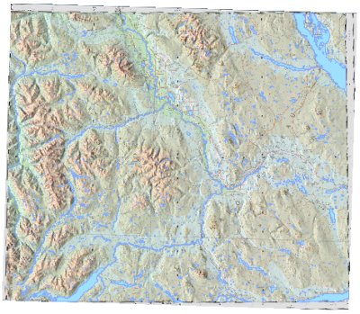
Add a masking region (white, no border) to obscure the grey margin
wedges. This is a region that is doughnut-shaped, with the inside
"hole" matching the map edges. This requires careful point-to-point
selection along the map
edges. If you have already made such a mask region for an adjacent map,
the quickest method is usually to make a copy, drag it over this map,
and then adjust all the points. Set the display style of this region
temporarily as no fill,
double -thick red border, and place at least 6 points along each edge.
Remove the display style override on the mask. Set the mapper to 20cm x
20cm. Window in to as close as possible around the map.
Save the workspace.
Saving final results
as PNG
Export (File|Save Window As...) as PNG, 24-bit, no border. 24-bit is
default, but "Export Border" has to be unchecked in the advanced
options). Specifically, if the mapper is 20cm wide by 20cm high,
export at 800 dpi. This results in a final
metres-per-pixel value of about 30.
It is important to leave the 24-bit colour depth. We tried reducing it
to an 8-bit paletted image to reduce file size, and on any given map
the difference was barely noticeable. However, when mosaicking adjacent
maps it became apparent that colours do not match up consistenly across
map edges with the 8-bit versions.
Save the workspace.
Saving final results
as Geotiff from MapInfo
Use Discover to save the window as registered raster. Make
the window 20x20 cm, and then go Discover|Map Window|Save As Registered
Raster. Use TIF, 8x and check Create World File. Call it <map
number>_shaded_relief. It should be about 6000x6000 pixels.
Merging in MapMerge
- Check the checkbox for the folder where the shaded relief maps
are. (It may be necessary to add this folder to the list)
- Note the pixel scales of the maps you want to merge. They should
be similar.
- Go to the Destination Map tab and
- set Pixel Scale to the largest of the pixel scales you are
merging. (It can be another value, such as an avergage scale, but this
guarantees you have downsampling rather than interpolation)
- set Zone
- Select the maps to merge by checking their boxes
- Click Create Map |From
Selected Maps
- Give a name for the saved merged mosaic
- Go for coffee (it takes a long time)
Remaining issues
Need to calibrate
final result
At this point it is necessary to take the PNG image into OziExplore and
calibrate it. While this is
not terribly time consuming, it introduces another possible source of
error.
It should be possible to export
the map as a GeoTiff that OziExplore can
read and automatically calibrate.
For OziExplore to read Geotiff, it must have the OziGeoTiff.dll file in
its install folder. You can get this (as ozigeotiff.zip) from the
oziexplore site (Optional Extras page)
Mosaicking final
results
Mosaicking the final maps with MapMerge generally works as well as
mosaicking PNG-format 250K topos distributed by Etopo. However,
sometimes (e.g., between 093F and 093K) there is visible gap of a
hundred metres or so.
Because these VNC-like topos are close in pixel dimensions to the Etopo
maps, it is likely this error arises in the calibration process.
I had a preliminary report that calibrating the maps in Lat/Long (as
opposed to UTM) produced better results. This has to be explored
further...
Apparent topographic
reversal
The maps are easy to read, even for people who have trouble
interpreting contour lines. However, an artifact of the shaded reliefe
is that if you turn the map around (place north at the bottom), the
relief also appears to invert. Valleys become ridges and ridges become
valleys. A bit of training and practice is required to attune the eye
to this effect.
Lakes obscure some
map text
Because we overlay the opaque water body regions on the map as the
uppermost layer, any text on the original map that runs across lakes is
lost. Generally this seems inconsequential, but there could be cases
where an important lake name is lost. It would certainly be possible to
review each map and position text on it to replace obscured water body
names.
Within BC, free data is available called the "Water Supply
Atlas." It contains a layer of all the text objects present on the
1:50,000 maps. This might be a useful resource.